This post is regarding an analysis which I performed as part of Kaggle Competition. It was a competition posted by Prudential Life Insurance company to help the organization to streamline the Insurance premium calculation process.

Scenario

In a one-click shopping world with on-demand everything, the life insurance application process is antiquated. Customers provide extensive information to identify risk classification and eligibility, including scheduling medical exams, a process that takes an average of 30 days.

The result? People are turned off. That’s why only 40% of U.S. households own individual life insurance. Prudential wants to make it quicker and less labor intensive for new and existing customers to get a quote while maintaining privacy boundaries. By developing a predictive model that accurately classifies risk using a more automated approach, you can greatly impact public perception of the industry.

Business Objective

The objective is to develop a predictive model that accurately classifies risk using a more automated approach. The Risk denotes the chances for a person to claiming his/her life insurance policy from the company. The Risk level helps Prudential Life insurance in providing an exact Quote of Life Insurance for each individual.

This will greatly help in public perception of the industry. The results will help Prudential better understand the predictive power of the data points in the existing assessment, and make the Life insurance process quicker and less labor intensive.

Dataset source:

• File Name : Train.csv
• Source of Data : https://www.kaggle.com/c/prudential-life-insurance-assessment/data
• Total No of Rows : 59381
• Total No of Variables : 128
• Time Period : NA (The time period is not mentioned on the source website)

Identifying Variable

Response Variable (Y):

The ‘Response’ field in the dataset is the dependant variable. ‘Response’ variable denotes the level of risk associated with a person’s chances of claiming his/her life insurance, in order to get a life Insurance Quote. This helps the Insurance company in assessing the application and denoting the right quote for the applicant. The several levels for ‘Response’ variable are: 1,2,3,4,5,6,7,8, where 8 means the highest level of risk. For example, if insurance risk level is calculated as ‘8’ for an individual, he/she has maximum chances of claiming insurance from the company, Therefore a level of 8 is bad for the insurance company

Predictor Variable (X):

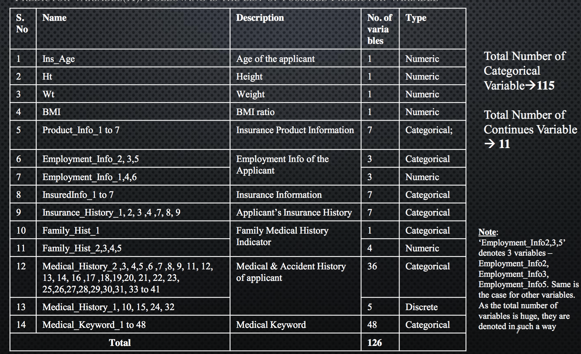
Following is the list of possible predictor variable

R Libraries

Following are some of the libraries which will be used in this analysis 1. library(nnet) ..Used to build the multinomial logistic model ..Uses the predictor variables to build a model which fits value for the Response variable 2. library(xlsx) ..To extract xls file into R ..Use to create the final output file in an excel sheet

Exploratory Analysis

In order to explore the data and develop a good regression model, 3 factors need to be understood:

1. Treating Missing Value
2. Feature Scaling
3. Association or Correlation between variables

A) Treating Missing Values

4 variables found to have missing values. The missing values are replaced with the ‘mean value’ of that column. The mean for the rows having not null value is calculated and updated where the value is missing.

B) Feature Scaling

Feature Scaling is a process where we standardize the range of values for independant variable. In some cases the range of values for a varibale is quite scattered, this makes it difficult to understand the relation of the independant variable with the Response variable. Fortunately, all the variables provide by prudential were already standardized. Therefore, we can skip this step all together and move to the next step.

C) Association or Correlation between variables

Categorical Variables

In order to determined if the Response variable(which is a Categorical variable) is dependant on any of the possible categorical predictor variable, following techniques can be used:

*Frequency Tables *Chi-square Test

The list of possible predictors are listed above. Out of these 115 are Categorical Variables

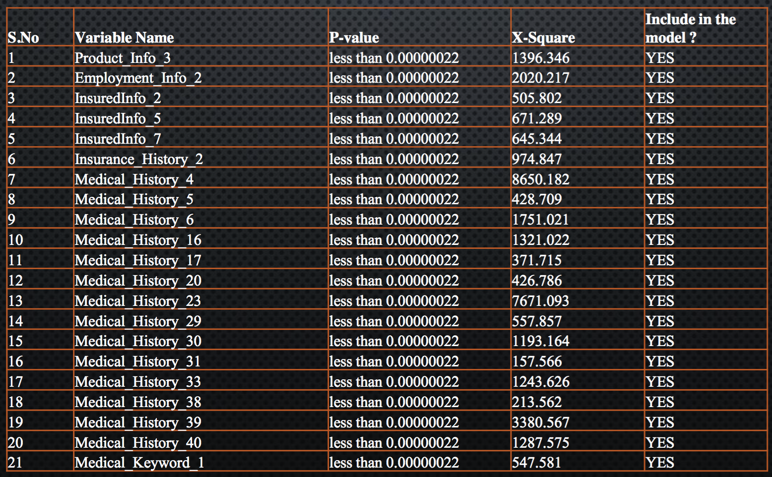
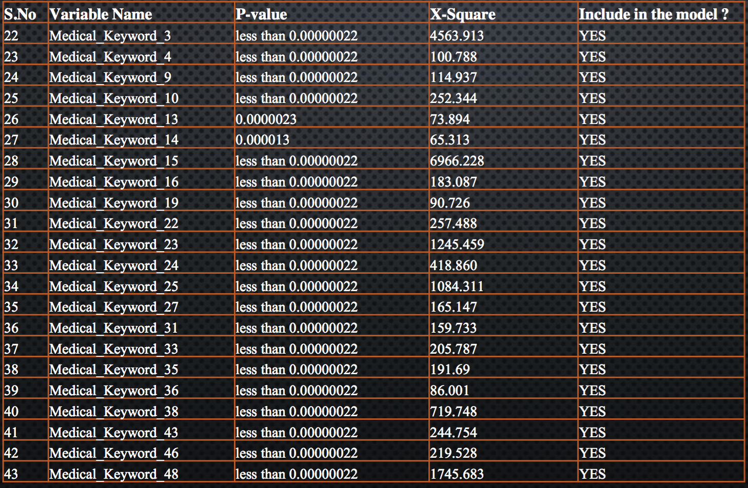
Out of 115 categorical variables, only 43 qualified the Chi-square test and have P-value less than 0.05. Following is the table which represent the P-value for each variable

Continous Variable

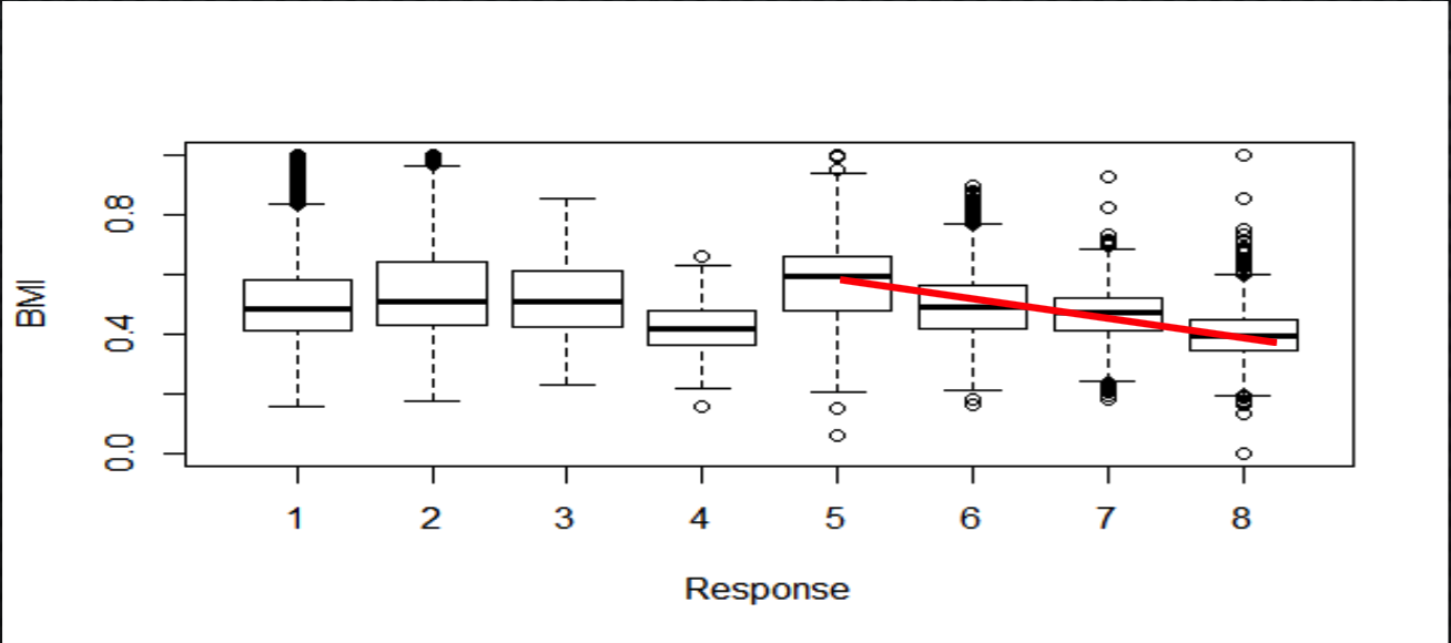
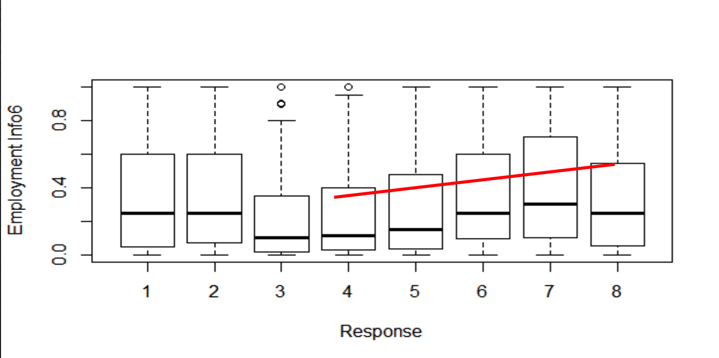
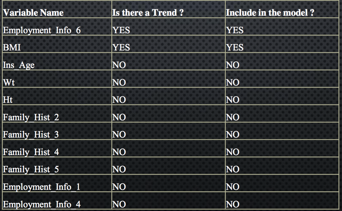
In order to understand the relation between continues independent variables and Response variables, we can use box plots. Out of 11 Continues variables, following 2 displayed a trend with the response variable *BMI *Employment Info 6

Following is the Box plot for Response variable and BMI, to understand the relation between them. The line highlighted in Red displays the trend between BMI & Response. As there is a trend for Response this variable can be included in the analysis

Following is the Box plot for Response variable and Employment Info 6, to understand the relation between them. The trend between the Response and Employment Info is denoted by the red line. As Employment Info has varied valued for each response category, it can be included in model.

List of table specifying which all continues variable to be included in the model

Regression Modelling Results

Building the model

• For this analysis, Multinomial Regression model is used. Multinomial Regression Model, is used to build a regression model where the response variable has more than two category. It is a generalization of the Logistic regression model.
• After exploring the data by identifying the best predictor variable and finding out the appropriate regression modeling technique. Next step is to build the model.
• The ‘multinom()’ function is used to build a regression model in R

Analyzing the model

• Following is the part of output for the summary of model
• The below screen shot denotes the Intercepts and coefficients for some of the variables in the model

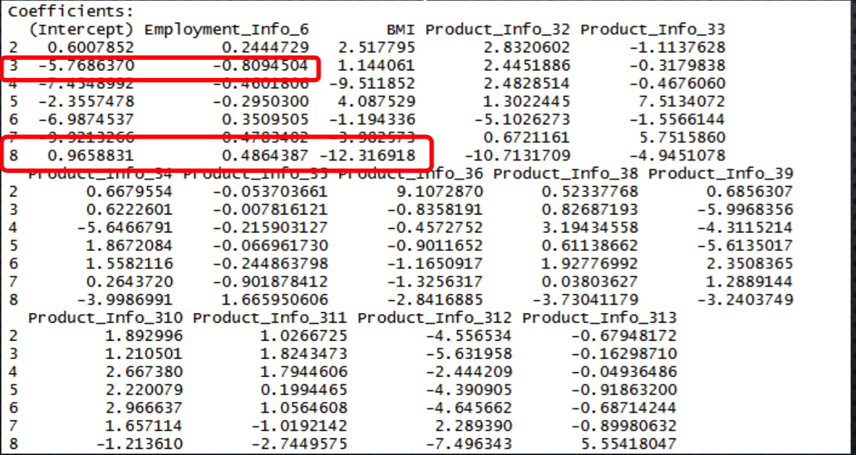
• The highest coefficient for BMI is for Response variable level – 8

Predicting values

• After the model is fitted, probability is calculated for each response type. The function ‘predict()’ is used to calculate the probability using the model on Test database
• A part of the output of the ‘predict()’ is a matrix, as displayed below

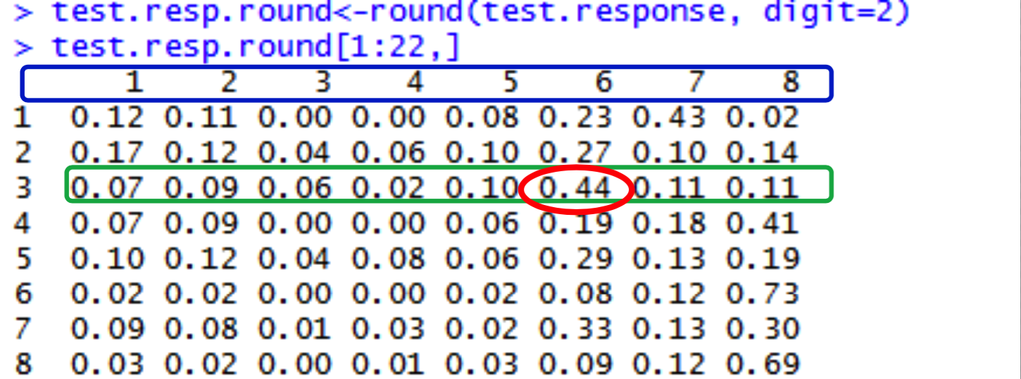
The above screenshot displays the output of the ‘predict’ function. The digits highlighted in blue are the Level of Risks(which we want to predict). The values circled with green denotes probability, of record no. 3, for each level of risk. For each record, the level for which the probability is highest is the final Level of risk. For example, record no 3 has highest probability for risk level 6, therefore record no 3 has predicted Level of risk as 6.

Conclusion

• The ‘Response’ variable for Test data set was predicted successfully using the following 45 predictors variables(43 Categorical & 2 Continues):
  • BMI
  • Employment Info6
  • Product Info3
  • Insured Info2,5,7
  • Medical History 4,5,6,16,17,20,23,29,30,31,33,38,39,40
  • Medical Keyword 1,3,4,9, 10,13,14,15,16,19,22,23,24,2527,31,33,35,36,38,43,46,48
• Note: ‘Insurance_Info2,5,7’ denotes 3 variables – Insurance_Info2, Insurance_Info5, Insurance_Info7. Same is the case for other variables. As the total number of variables is huge, they are denoted in such a way
• The response variable denotes the level of risk associated with the Life insurance of a particular individual. Most frequent value for Response is ‘8’ in the test data. Therefore the most occurring risk is level 8 for the output data set.
• The predictor variable BMI has the strongest positive correlation with the ‘Level of Risk’, therefore we can conclude that a change in the BMI level significantly changes the ‘Level of Risk’ of a life insurance applicant.